NEID Pipeline Algorithms
CCD Image Processing
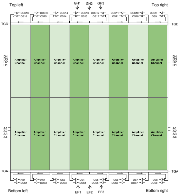
The Level0 raw data is assembled into 2D images in this step. The NEID e2V 9kx9k detector is read out in 16 channels as shown in the image at right. There are overscan, prescan and post readout regions (defined by BIASSEC1, BIASSEC2, and BIASSEC3 keywords) for each readout channel. The prescan, overscan and post readouts regions are collapsed to 1D vectors by biweight averaging. This average vector for each amplifies is further smoothed by an Savitzky-Golay filter of window size 9, and degree 2 before subtracting from the detector pixels.
Finally, the overscan and pre-scan corrected channels are assembled into the 2D image frames and saved as temporary files neidTemp_2D*.fits. The variance image array is also generated for propagating through the pipeline at this stage by combining the photon noise and detector readout noise. These 2D images are not retained after DRP runs complete; they are large in size (~650 MB/image) and do not contain unique, or difficult to reproduce information.
Calibration images are then inspected relative to a nominal flux standard. Frames which are severely devient, for example due to a failing lamp, are identified an not used in subsequent pipeline steps.
A static badpixel mask is then applied to each image; bad pixels are set to NaN, and treated accordingly throughout the remainder of the pipeline. This mask removes several obvious hot column features in the left top and bottom amplifiers, as well as several other more subtle hot pixels and readout defects that were measured emperically in CCD.
Flat field preparation
The NEID CCD is covered in a thin layer of ice, which is changing over time. Consequently, flat fielding must have a temporal component. The DRP derives custom, individual flats for each exposure based on when it was taken.
This process begins by preparing the master flat files. The Flat2D files from the morning and evening cals are combined separately to form two high SNR Flat2D frames. These frames are then normalized by a template illumination pattern from the second half of March 2021. A Master 2D flat, consisting of a pixel by pixel linear model, is constructed from the two normalized frames. The fiber continuum lamp Master flats of LDLS and FlatBB are also created in a similar manner. No flat correction or normalization is done for the continuum lamp spectrum. The individual frames are scaled to a common value in each fiber before averaging to correct for any small differences in effective shutter open time. A scattered light subtraction is done to remove scattered light while generating the individual continuum lamp master flats for each fiber. Similar to Flat2D, a fitted linear model is constructed and saved from the morning and evening cal sets.
The master flats are then interpolated to the epoch of each science frame.
Scattered light correction
The Scattered light in the frames to be extracted are corrected in a two step process.
Template based correction of the light source in other fibers: If the light source in the other two fibers are Etalon, ThAr, LDLS, FlatBB, Sun or Star, a high SNR master template frame of this lamp source is fitted to the data and subtracted. This subtraction corrects for the high frequency fiber to fiber cross contamination in the 2Dimage from these sources.
2D Spline fit for the diffuse scattered light: The pixels which are significantly away from the fibers and which contain any light source are used to fit a 2D spline. The knots of the 2Dspline are chosen such that they have higher resolution in cross dispersion direction, and lower resolution in dispersion direction.
Spectral Extraction
Continuum Sources
For stars and other non emission line calibration lamps, we use flat relative optimal extraction (Zechmeister et. al. 2013). The photon noise from the subtracted scattered light is not considered in the variance weighting of the optimal extraction calculation. This is to prevent scattered light dependence in an unresolved emission line or absorption line profile in the spectrum. Echelle orders bluer than 6450 A are extracted using the interpolated LDLS flat, and the echelle orders redder than 6450 A are extracted using the interpolated FlatBB flat frames. Output of flat relative optimal extraction provides the extracted spectrum relative to the lamp’s spectrum. This is corrected in the later stage of the pipeline.
Line Emission Sources
For emission line calibration lamp sources such as the Etalon, LFC and ThAr, NEID’s circular fiber results in a profile mismatch at the edges of the line compared to the cross dispersion profile derived from a continuum flat lamp. This results in a flux dependent bias in the averaging weighting used in optimal extraction. In order to prevent a flux dependence in the line profile shape of unresolved emission lines, we fall back to flat relative non-optimal extraction. In conventional optimal extraction, the independent estimates from each cross dispersion pixel are averaged using the weights proportional to the square of the cross dispersion profile and inversely proportional to the variance of the pixels. In our non-optimal extraction, we average using weights which are proportional to the cross dispersion profile. Mathematically, this is equivalent to a sum extraction of the spectrum divided by the sum extraction of the flat spectrum. Hence it does not have any aperture edge artifacts or missing bad pixel impacts seen in a conventional sum extraction.
Cosmic Ray Rejection
Cosmic ray affected pixels are rejected iteratively inside the extraction step described above. Due to the mismatch in the cross dispersion profile obtained from a continuum flat, on the edges of unresolved emission lines like Etalon, LFC, and ThAr, we do not use conventional cosmic ray rejection algorithms. Instead, the following algorithm is used to identify and mask out the pixels affected by cosmic rays one echelle order at a time.
The flux estimated from the first iteration of flat-relative optimal extraction is used to scale the flat spectrum to the stellar spectrum.
A sigma image is formed by subtracting the stellar spectrum frame with the scaled flat spectrum inside an echelle order, and dividing it by the sigma of the noise at each pixel.
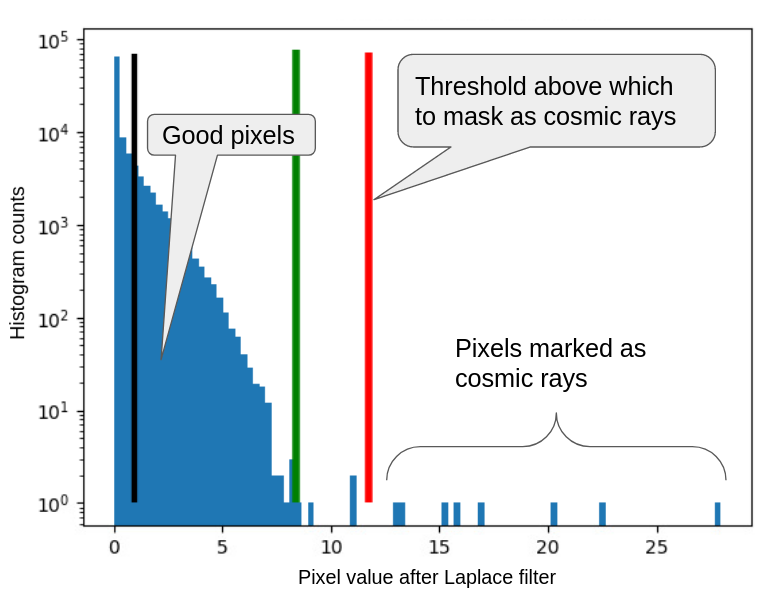
To identify cosmic rays, this sigma image is up-sampled and a negative laplace filter is applied. Negative values are clipped to zero, before downsampling the laplace filtered images back to original size.
An extrapolation is done in percentile values to obtain a robust upper limit on the distribution of these pixels. The figure at right shows a typical histogram, the green line marks the upper limit of the good pixels estimated, and all the pixels with values larger than the red marker are treated as cosmic ray pixels.
After the cosmic ray pixels are masked the extraction is redone to obtain a new flux estimate and the process is repeated until no new pixels are marked as cosmic rays.
Variance Correction
While calculating the variance in optimal extraction the photon noise from the subtracted scattered light is not considered. This contribution to the variance of the extracted spectrum is added back by sum extracting the photons in the subtracted scattered light model.
Final Units
The spectrum of the continuum lamp used for the flat-relative extraction needs to be multiplied back to obtain the final extracted spectrum in units of e- ‘s collected in the exposure time. The interpolated continuum lamp spectrum used for flat relative extraction are first divided by normalised Flat2D. This corrects for the low frequency chromatic QE changes across the time. This frame is then sum extracted to obtain the continuum lamp spectrum corrected for QE changes. A smooth template model of the continuum lamp spectrum is then fitted to this data to obtain a noiseless and flat corrected spectrum. This final model of the continuum lamp spectrum is then multiplied to the flat relative (optimal or non-optimal) extracted spectrum to obtain spectrum in units of e-.
Fallbacks
In the event of failed daily cals, where there are no continuum lamp flats available the pipeline will fall back to sum extraction with no flat correction.
LDLS Fringe Correction
A filter in the LDLS produces a sinusodial fringe on the order of 200 pixels in all extracted data. This fringe is daily variable in both amplitude and phase. Using a template model, the pipeline estimates a daily amplitude and phase from the calbration data. After extraction is completed, each L1 file is divided by the constructed Daily LDLS fringe model.
Wavelength Calibration
Wavelength calibration of the extracted spectra proceeds independently for each observing session (i.e. a solar day or a night), using a suite of calibration sources including a Laser Frequency Comb (LFC), a Fabry-Perot Etalon (FP), and a ThAr hollow-cathode lamp. The wavelength calibration for a given night is informed by a “master” set of calibrations, the standard pre-observing calibration data for that session, as well as monitoring and correction of instrumental drifts throughout the session.
Note: From July through December 2024 NEID’s Fabry-Perot Etalon was uninstalled for maintenance. During this time, the LFC is used for measuring the instrument’s daily drift.
Wavelength Calibration Sources
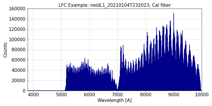
LFC: The Laser Frequency Comb provides a spectrum of modes with centroid frequencies known precisely and absolutely. The separation between these modes is maintained at a constant 20 GHz, which corresponds to roughly 4 resolution elements in HR mode. The LFC spectrum spans approximately 500nm through 930nm, so it does not provide wavelength information across the full NEID bandpass.
The LFC was upgraded in August 2024 to expand its spectral grasp down to roughly 420 nm (which still does not cover the full bandpass).
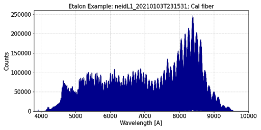
FP The Fabry-Perot etalon provides a spectrum of modes spaced by approximately 20 GHz from ~440nm-930nm. These modes are stable over the short term, but exhibit uncontrolled drift over timescales of weeks.
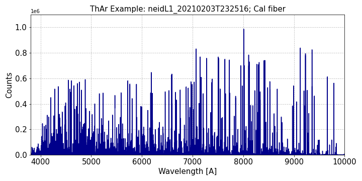
ThAr The Thorium-Argon hollow-cathode lamps have lines with well-known wavelengths across the NEID bandpass.
Laser Frequency Comb Quality Control
Frame-wise Quality Control
DRP v1.4.0 introduces quality control vetting of the laser frequency comb observations used for wavelength calibration at the full LFC spectrum level (frame-wise). Sometimes the LFC is unstable, causing significant variations in flux that impact the quality of the fits to LFC modes. When that happens, the issues with the mode fits trickle down to the wavelength solution, degrading its precision. It has been seen that these LFC flux stability issues can cause RV precision to decrease by 5-10 m/s.
We now vet the quality of each LFC frame based on the average FWHM of the Gaussians fit to all modes across the LFC spectrum. Significant flux variations lead to significant variation in the FWHM values, due to either vast drops in flux (fitting a Gaussian to noise) or vast increases in flux (fitting saturated lines).
LFC frames that fail vetting are not used in the wavelength calibration, leading to better wavelength solutions and improved RV precision. See NEID RV Eras and the RV time series plot shown there for an example of how the vetting has improved RV precision.
Individual Mode-wise Quality Control
DRP v1.5.0 introduces quality control vetting of the individual modes in an LFC observation (mode-wise). When the LFC flux is unstable, it is possible that some modes in an order have high signal-to-noise while other modes (particularly outside of the free spectral range) have severely degraded signal-to-noise. This can lead to individual orders having low precision wavelength solutions, biasing the overall RV measurement.
We now perform multiple levels of refinement to each order’s wavelength solution fitting (see below for details) that include only using LFC modes that pass a set of vetting criteria to ensure they have sufficient signal-to-noise for well-measured centroids.
Daily Wavelength Calibration
Our wavelength calibration routine depends on a standardized calibration observation sequence that is executed during each of our calibration sessions (evening calibrations for nighttime data, morning calibrations for solar data). During these sequences, spectra are taken of multiple wavelength calibration sources: the LFC and FP in each fiber, as well as a hollow cathode lamp spectrum (ThAr, with UNe beginning in August 2023).
For both the LFC and the FP, each individual modes across all orders with calibration light are independent fit in pixel space using an unweighted least-squares fit of a Gaussian function. The results are recorded in diagnostic files with tables of various fit result information per mode.
Base Wavelength Solution
The first major step is to generate a base wavelength solution during the wavelength calibration session. This represent’s the instrument’s wavelength solution in each fiber at the epoch of the calibration sequence. We later apply drifts to this base wavelength solution to generate a wavelength solution at any time during the observing session (see the below section Within-session Drift Correction for more information.)
The NEID wavelength solution incorporates information from the LFC
calibration sequence spectra and a master wavelength solution based on
ThAr spectra. As of DRP v1.5.0 there are 3 different types of base
wavelength solutions that can be generated by the pipeline. The type
used is denoted by the WAVECAL header keyword, and each uses a
different combination of LFC/ThAr information and thus a different
expected precision level.
It is possible for each fiber to have a different wavelength calibration
algorithm applied. The WAVECAL keyword that appears in the Level 1
and Level 2 primary headers represents the wavelength calibration used
for the Science fiber. There is a WAVECAL keyword in each of the
fiber wavelength extensions that denote the algorithm used for that
fiber.
These algorithms are described below:
LFCplusThAr
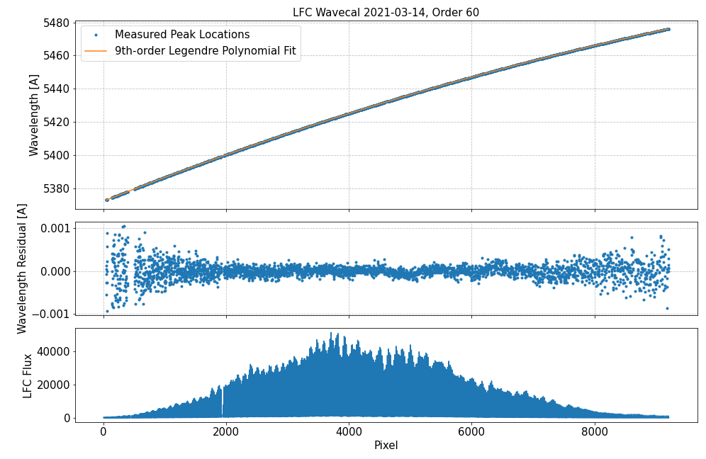
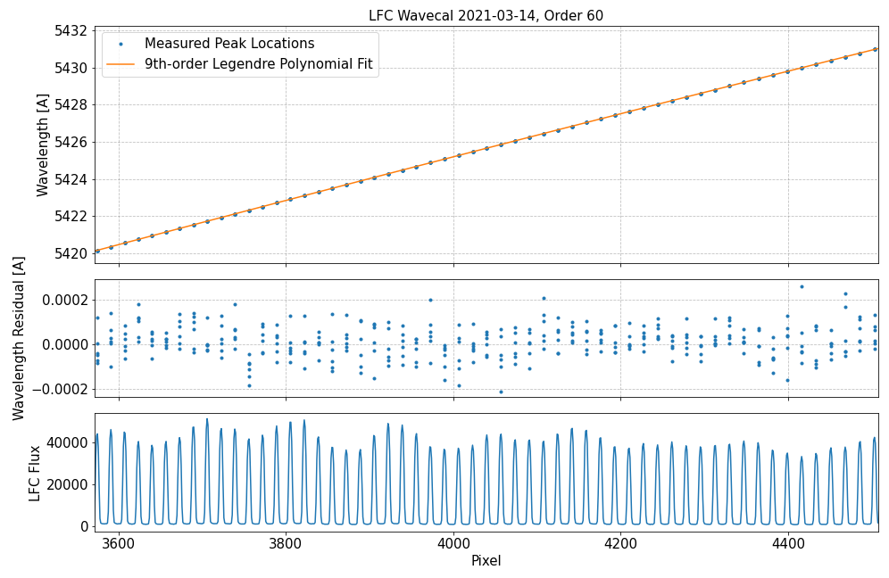
In this wavelength calibration scheme, the fit centroid pixel for the LFC modes are combined with the known LFC mode wavelengths to inform a least-squares fit of a 9th-order Legendre polynomial to generate a wavelength solution for each spectral order with LFC light. These fits are performed independently for each spectral order and for each fiber. The wavelength solution polynomial fits incorporate all LFC modes in an order that are successfully fit with Gaussians and use the master ThAr-based wavelength solution as an initial coefficient guess.
The LFC-based wavelength solution undergoes additional rounds of fitting for further refinement:
Mode Vetting Refinement: First, the wavelength solution is re-fit using only LFC modes that pass vetting criteria on parameters about each individual mode fit. These criteria include making sure the mode has a positive amplitude, a reasonable width, a peak signal-to-noise above 3, and a pixel centroid error that is not unreasonably large. This refinement greatly improves the quality of the wavelength solution when the LFC is experiencing flux instability.
Free Spectral Range Refinement: Next, the zero-th order coefficient of the wavelength solution is re-fit using only LFC modes that both pass the per-mode vetting from above AND are within the order’s free spectral range. Restricting to this range ensures only the highest signal-to-noise modes are used in the fit, but gives little leverage for the high order coefficients. This refinement further improves the wavelength solution when the LFC is experience flux instability, and appears to improve quality even when the LFC is well-behaved.
Prior to 8/26/2024 the LFC is used to derive wavelength solutions for zero-indexed orders 58 through 110. After that date, the LFC is used to derive wavelength solutions for zero-indexed orders 40 through 110.
(Note: prior to DRPv1.4.0 the LFC was used to derive the wavelength solution for zero-indexed orders 55 through 110. Orders 55-57 were changed to use the drifted master ThAr wavelength solution in DRP v1.4.0 due to flux instability in those orders. The change in which orders use the LFC is one cause for RV offsets between versions of the DRP.)
The wavelength solutions for orders without LFC light are generated from the master ThAr-based wavelength solution. The fit LFC mode centroid pixels are compared to their centroids at the epoch of the ThAr-based master wavelength solution. The ensemble of per-mode centroid differences is used to define a single velocity drift from the ThAr epoch to the observing session being calibrated. This zero-point drift is applied to the ThAr-based master wavelength solution and used for all orders outside of the LFC range.
Each fiber has a separate zero-point drift. This zero-point drift is
saved in the ZPTDRIFT header keyword in the wavelength extensions of
NEID Level 1 and Level 2 data. (All observations on a given night will
have the same ZPTDRIFT value.)
A session calibrated with this LFCplusThAr algorithm is the highest precision calibration currently available in the NEID DRP.
LFCplusThArModified (Introduced in v1.5.0)
This wavelength calibration scheme largely follows the LFCplusThAr scheme, but is used when an order with an LFC wavelength solution is identified as having a bad calibration.
An order is called “bad” if more than 60% of the individual LFC modes in it fail the per-mode vetting. In this case, the wavelength solutions for the bad orders are generated using information from the wavelength solutions from other orders.
The lower order polynomial coefficients (0th-4th order) for a bad order are replaced by evaluating a “hyper-fit” to each of those coefficients as a function of spectral order. These “hyper-fits” include information from both well-calibrated LFC orders and the ThAr-based master wavelength solution.
The higher order polynomial coefficients (5th-9th order) for a bad order are replaced by the median value across the redder set of LFC orders. These higher order coefficients are found historically to be quite stable across order.
If this calibration scheme is used, the orders identified as bad are listed in the HISTORY entries of the L1 and L2 wavelength extension headers for each fiber.
A session calibrated with this LFCplusThArModified algorithm should still be usable for high precision science. This scheme is largely used when the LFC flux is unstable over a small portion of its bandpass (typically the blue end), particularly over various spans of time from August 2025 onwards. However, we encourage users to carefully inspect their data when this calibration scheme is used. Further investigations by the instrument team will be performed to quantify the expected precision of this scheme.
ThAronly
In this calibration scheme, the base wavelength solution is simply the ThAr-based master wavelength solution. This is triggered only when there are no LFC calibration frames available for a given fiber.
A session calibrated with the ThAronly scheme cannot be used for high precision science. Depending on the observation time (essentially how far has the instrument drifted from the epoch of the ThAr master) can have maximum precisions of only 10s to 100s of m/s.
Within-session Drift Correction
The instrumental drift throughout an observing session must still be corrected. This is presently represented purely as a velocity shift, and there are multiple possible methods for estimating and interpolating the value of this velocity appropriate to a given observation. In each case, the interpolated velocity is used to transform the nightly wavelength solution for each fiber, and the result defines the wavelength array for that epoch.
The measured velocity shift is implemented as 1 / (1 + v/c) and is
stored in the primary header of Level 1 and Level 2 data (DRIFTRV0).
This represents the velocity shift used within the night, and should not
be compared across nights.
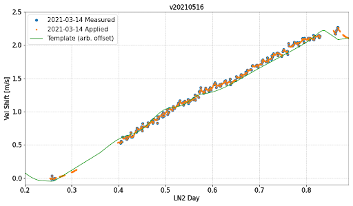
DailyModel (default) - This method invokes the measurement of calibration source modes in standard calibration-fiber exposures throughout the observing session (such as those taken in “bracketing” exposures, as well as simultaneously recorded with Solar spectra, for example). Each ensemble of mode measurements is compared to the same information from the pre-calibration standard exposures, and used to define a single velocity shift for that time. As of DRP v1.4.0, only modes that fall within the instrument’s free spectral range are used to measure the drift – this increases the robustness of the drift measurements to poor mode line fits (such as from reduced flux). The resulting set of (times, velocities) is then interpolated using the master drift template, with weighting decreasing from the time of interpolation. Either the FP or LFC can be used to measure this drift. The FP is used prior to July 2, 2024 and after March 31, 2025. From July 2024 through March 2025 the LFC is used. As of DRPv1.1, this is the default method for both nighttime and solar data where sufficient calibration data exist.
Constant - In this case, the velocity shift is taken to be 0 for all observing times throughout the observing session. The nightly calibration thus becomes the constant wavelength array for the entire session. In this case, radial velocities are at best precise to the few m/s level.
Master - In this case, the master wavelength calibration is used. This involves no translation for the instrumental drifts between the time of the master and the observation, nor for the drifts within the observing session. This is typically the only method that is possible for observing sessions where the LFC is compromised. In this case, radial velocities are at best precise to the 10s - 100 m/s level.
Depreciated Drift Functions
The following drift functions are no longer used as of DRP v1.4.0.
Linear - Similar to DailyModel, this method uses the FP mode fits from the post-observing calibration exposures to define a velocity shift between the pre and post-observing times. These values are linearly interpolated onto any observation time in between.
Simultaneous - Again, the ensemble of FP mode fits defines a velocity shift from the pre-observing calibrations, but in this case only information from contemporaneous calibration FP data are used. This method is only possible for data where the FP illuminates the Cal fiber.
Header Information
Information about the wavelength calibration process is conveyed in several header keywords.
WAVECAL This corresponds to the wavelength solution generation algorithm used, which are described in sub-sections above. Each fiber’s wavelength extension has its own
WAVECALkeyword, and the keyword in the primary header is theWAVECALof the science fiber.DRIFTFUN This corresponds to the drift function options listed above. This only exists in the primary header.
PS[N]_0 This describes the polynomial type used to fit the wavelength calibration for order N. Default is currently “Legendre”.
PS[N]_1 This lists the number of parameters used in the polynomial. (i.e. the order of the polynomial)
PS[N]_2 This describes the domain of the polynomial. (i.e. range of pixel values)
PS[N]_3 This describes the window of the polynomial function. (i.e. range of input for polynomial)
PV[O]_[N] This is the value of the polynomial parameter N for order O.
ZPTDRIFT This is the zero-point drift value used if the
WAVECALis either LFCplusThAr or LFCplusThArModified. This exists in the individual fiber wavelength extension headers (added v1.5.0).
Note: As of DRPv1.1 the wavelength polynomial coefficients are consistent with the wavelength calibration of each spectrum. In previous versions, these coefficients were inaccurate.
Fallback and Wavecal Quality
There are two main reasons for why the wavelength calibration may fallback to lower quality in the above described calibration scheme:
Missing LFC: The LFC is unavailable on some days, making it impossible to derive the wavelength solution or an accurate velocity shift relative to the ThAr master solution for that observing session. In these cases the wavelength calibration falls back to
ThAronly, where we simply insert the ThAr-derived master wavelength solution for all data that day.Missing Drift Monitoring Data: In other cases, there may be sufficient LFC data in the calibration session to define the wavelength solution for the night, but insufficient drift monitoring data to measure drifts throughout the night (either FP or LFC depending on the date). In these cases the wavelength calibration falls back to
CONSTANT, where we insert the LFC+ThAr derived wavelength solution for that day for all data obtained.
Note
In DRP v1.5.0 we introduced a new WAVECAL
scheme called LFCplusThArModified. This will recover some nights that
had lower precision in v1.4.x during times when the LFC was flux
unstable despite having the gold standard WAVECAL keyword
LFCplusThAr.
Note
In DRP v1.4.0 we removed two causes of fallbacks that were not necessary. This means that there may be some nights in your data sets that previously fell back to low precision, but are now recovered. Please check your data to see if any nights have been recovered in DRP v1.4.0. The two fallback causes removed are:
1) Fallback to ThAronly if HR Sky Fiber LFC observations were missing
from the calibration session. HR-mode RV science observations only
depend on the Cal and Science fibers. Thus, this was an unnecessary
fallback that reduced the precision of otherwise good observing nights.
In this case, the Sky fiber wavelength solution falls back to the master
solution but the Science and Cal fibers do not. If you are interested
in using the Sky fiber, we note when this fallback occurs in the
HISTORY of the L1 and L2 FITS headers. Please look there before
proceeding with your analysis.
2) Fallback to CONSTANT if FP observations are missing from the
calibration session at the end of an observing session. As long as
enough drift monitoring observations are obtained at the beginning and
throughout an observing session, the DailyModel drift function can be
applied precisely. This largely affected nights where there were a lack
of HR Sky fiber Etalon observations.
For the highest quality wavelength solutions the WAVECAL and DRIFTFUN header keywords should be:
In DRP v1.1.0 and after: WAVECAL=LFCplusThAr and DRIFTFUN=dailymodel0 (in both nighttime and solar data).
In DRP v1.0.0: WAVECAL=LFCplusThAr, DRIFTFUN=dailymodel (for nighttime data) or DRIFTFUN=simultaneous (for solar data).
Observations with WAVECAL=LFCplusThArModified are likely usable for high precision science but should be treated cautiously. Observations with any other keywords (WAVECAL=ThAronly, DRIFTFUN != dailymodel0) should be treated with extreme caution and are unusable for high precision RVs.
Barycentric Correction
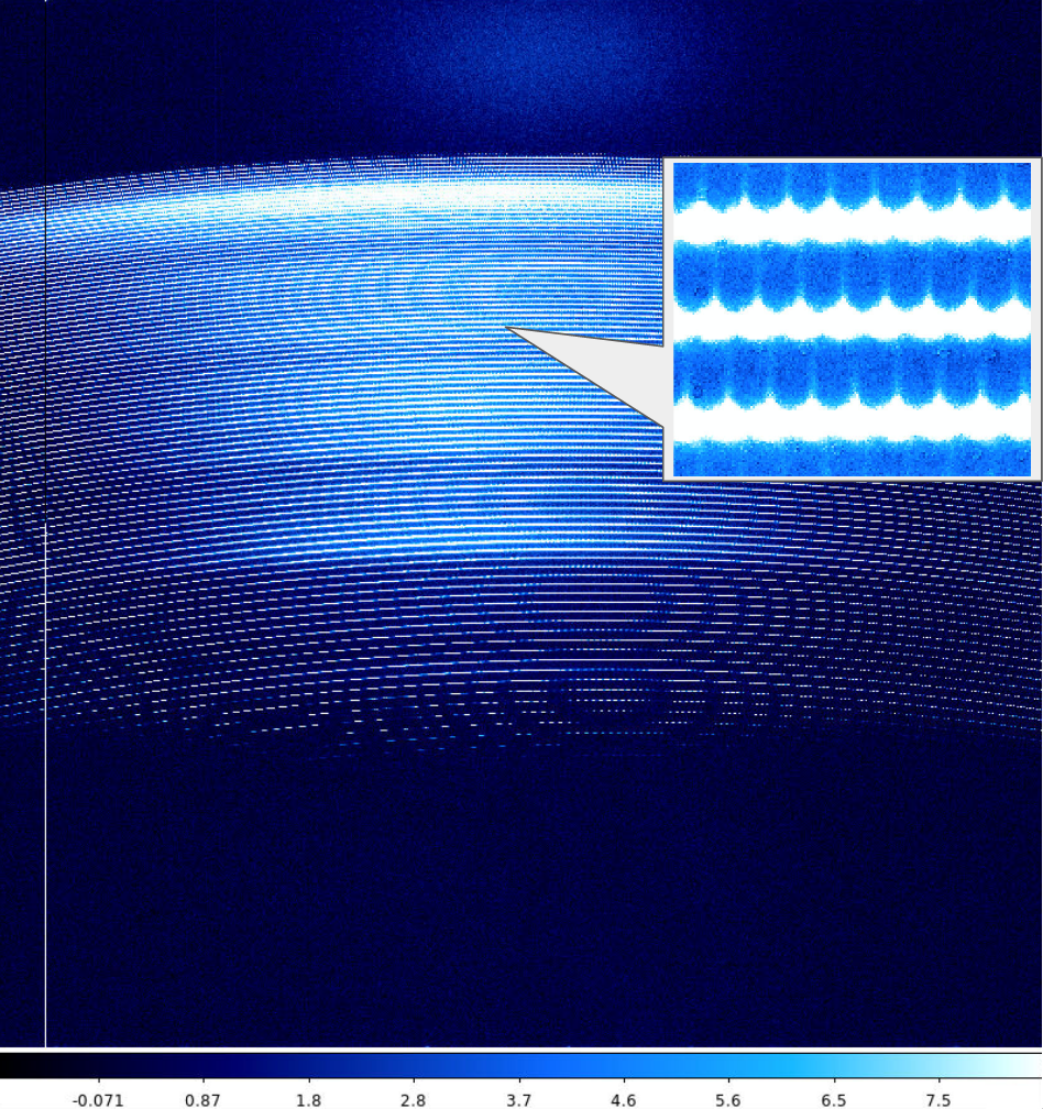
In order to perform the barycentric correction, we need to estimate the flux weighted midpoint for each NEID exposure as a function of wavelength. For this we use a chromatic exposure meter at 1 Hz cadence with 64 spectral bins. After filtering for cosmic rays, we subtract a bias frame from each exposure meter exposure, and correct for readout contamination due to the shutterless readout. After interpolating the spectrum to a common wavelength grid, we correct the optical cross talk between adjacent fibers. Using the fluxes from these corrected frames, we estimate a flux weighted midpoint for each grating order in NEID. The granularity of the flux wavelength bins in the exposure meter is adaptively adjusted to obtain optimal balance between the signal to noise ratio in each bin and the overall spectral resolution.
These midpoints are then input into barycorrpy (Kanodia and Wright 2018).
Stellar barycentric corrections
Barycorrpy implements the algorithms of Wright and Eastman (2014) using the flux weighted midpoint calculated from the exposure meter, and astrometry from Gaia DR2. The zb is calculated from barycorrpy using zmeas=0, and is associated with the BJDTDB time calculated using barycorrpy.
Solar barycentric corrections
Barycorrpy implements the algorithms of Wright and Kanodia (2020) to compute the barycentric correction for the Sun with zmeas=0. Used in the predictive mode, the code calculates zpredict, which is then converted into a barycentric correction (z_B_SS) as such - z_B_SS = 1./(1.+z_predict)-1. In this mode the barycentric correction output takes into account the motion of the Sun due to the solar system planets, and corrects for it using Eqn 10 from Wright and Eastman (2010). These outputs are time stamped with the HJDTDB computed using barycorrpy.
See the barycorrpy documentation on GitHub for further explanation.
Telluric Model
Telluric Model Grid
The telluric module utilizes a master grid of telluric models created with the AER Inc. LBLRTM line-by-line radiative transfer code. The telluric model grid was generated over the following dimensions:
Wavelength: 3570.8 to 11047.2 Angstrom
Zenith angle: from 5 to 75 degrees, in steps of 5 degrees
Precipitable water vapor: from 0 to 40 mm, in steps of 5 mm
This results in a set of 135 grid points total, one for each pair of zenith angle and precipitable water vapor value. At each grid point there are two absorption models generated: one with just line absorption and one with just continuum absorption.
In generating these models, LBLRTM was configured with the following parameters common to each type of absorption model:
Species up to O2 are used
HIRAC voigt profile is used (IHIRAC=1)
No aerosols are used (IAERSL=0)
Radiance and transmittance is used (IEMIT=1)
The atmospheric profile is scaled up to H20 (NMOL_SCAL=1)
The scaling factor is computed in units of cm of precipitable water vapor (HMOL_SCAL=P)
The U.S. standard 1976 is used (MODEL=6)
For the line absorption models, the following parameters are used:
Line by line bound is set to 25 cm^-1 for all layer pressures (LBLF4=1)
For the continuum absorption models, the following parameters are used:
All continua are calculated, including Rayleigh extinction (ICNTNM=1)
The LBLRTM output models are rebinned to a common wavelength grid that is coarser than the LBLRTM output but oversampled relative to NEID. The master file telluric model wavelength grid is equally spaced in log-wavelength.
Telluric Model Fitting Routine
The telluric module fitting routine takes an in-progress Level 2 file as input and uses the above described model grid to fit for a precipitable water vapor (PWV) value. The routine fits the model grid to multiple distinct spectral regions that are defined in the neid_telluric.config file. The module has functionality to fit any arbitrary number of spectral regions (which are defined as a list of wavelength extents for each region in the config file). The input data flux array is deblazed. The fitting routine steps are:
1. The telluric model grid is interpolated to the zenith angle of the observation. For night-time observations the zenith angle is calculated from the airmass value in the primary header. For solar observations it is calculated using astropy.coordinate’s get_sun function. This leaves PWV as the only free parameter.
2. For each spectral region used in the fit, the data wavelength and flux are taken from the spectral order with a median wavelength closest to the middle of the fit region. The chunk of data wavelength and flux within the defined spectral region are taken for use in the PWV fit.
3. We then process the zenith-interpolated telluric model grid for each fit region. At each PWV grid point, the chunk of the zenith-interpolated model within a particular fit region is convolved with the NEID line spread function (LSF). The LSF is variable and defines a unique convolution kernel at each wavelength. We describe the LSF in the next section. The convolved model is then rebinned to the data wavelength values in the fit region.
4. A least-squares fit for PWV is then performed by interpolating the convolved and rebinned model grid at varying PWV values and comparing to the input deblazed data spectrum. If multiple fit regions are used, the least-squares is calculated using all regions simultaneously. Using multiple regions helps to minimize the effect of stellar lines contaminating the fit and biasing the fit PWV to higher values (depending on the Doppler shift of the stellar lines in the region).
5. The main telluric model grid is interpolated to the zenith angle and best fit PWV to generate the output Level 2 telluric model. For each spectral order, the interpolated telluric model within its wavelength extent is convolved with the variable LSF and rebinned to the observed data wavelength values. Orders containing invalid wavelength values are ignored and the output model is set 1. Orders without a defined variable LSF have their output model set to 1 (outside orders 55-110, zero-indexed). This step is performed twice: once each for the line and continuum absorption model grids.
In v1.3.0, tested and deployed at the end of August 2023, the spectral regions included in the telluric fit are: 5945 - 5950 A, 5968 - 5974 A, 6486 - 6493 A, 7075 - 7083 A, 7247 - 7252.5 A, 7354.5 - 7359.5 A (this last region was the sole region used in DRP v1.1 and 1.2)
The output telluric model in the Level 2 file has dimensions: number of orders (122), number of dispersion pixels (9216), 2. The last axis contains the separate line and continuum absorption models. Index 0 contains the line absorption and index 1 contains the continuum absorption. A full telluric absorption model is obtained by multiplying the two together.
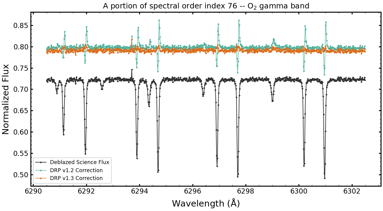
The plot to the right shows an example result of the telluric model fitting routine for an A-star standard observation. The region shown is a zoom-in on the O2 gamma-band, which highlights how the use of the variable LSF improves the model.
While there are still small structured residuals in the new model correction (orange), the residuals are dramatically improved from the DRP v1.1/1.2 model correction (teal). There are also three weak water lines in this region at 6294.25 A, 6296.4 A, 6299 A. The correction is improved in DRP v1.3 compared to DRP v1.2, a result from the variable LSF and improved PWV fitting routine.
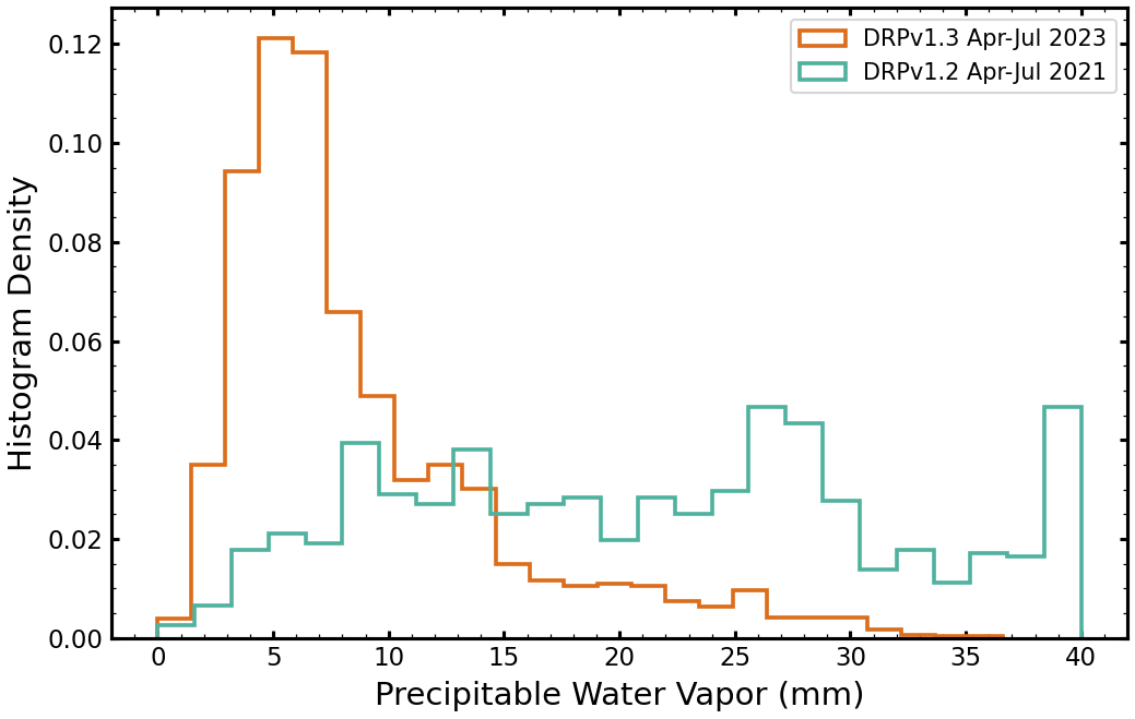
The plot on the left shows the histograms of precipitable water vapor values for DRP v1.2 fits of data ranging from April-July 2021 (teal) and for DRP v1.3 fits of data ranging from April-July 2023 (orange). The same span of months was chosen to compare data in similar seasons. The PWV values from the DRP v1.2 fits are significantly larger than the DRP v1.3 values, despite what should be comparable seasonal conditions (the humidity and zenith distributions in each data set are comparable).
The distribution of PWV values in the DRP v1.3 data set is more in line with expectations, and reflect the improvement in the telluric model fit by using multiple spectral fit regions (to reduce stellar line contamination that biases PWV to higher values).
Variable Line Spread Function
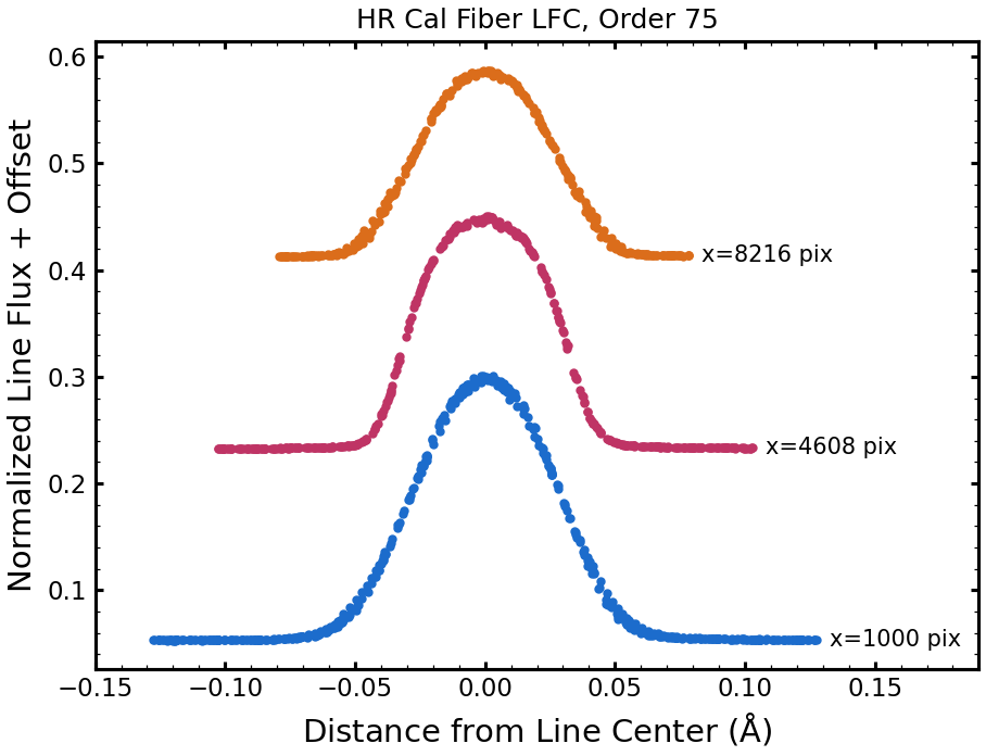
The line spread function is known to be variable across the NEID spectrum. It is necessary to convolve the above described LBLRTM-calculated telluric absorption model grid with a line spread function that is representative of the actual data to produce a useful telluric correction. The plot to the right shows three sets of stacked LFC lines in spectral order 75 from a NEID LFC exposure in the HR Cal fiber. From bottom to top as plotted, the three sets of LFC lines represent the blue end, middle, and red end of the order. The LFC line is intrinsically narrow enough that it is representative of the instrumental line spread function. It is clear in the plot that the line spread function is variable across the order in width and shape. The line spread function is variable from order to order as well.
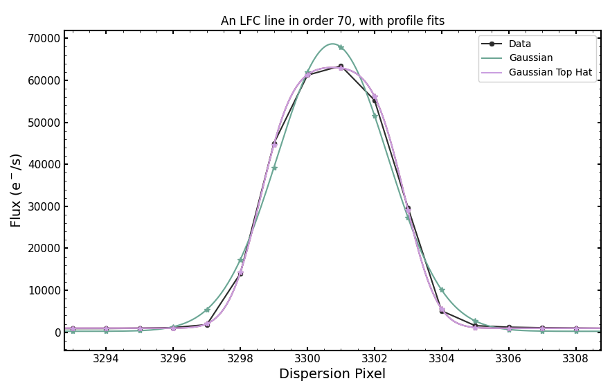
In DRP v1.3 (August 2023) we parameterize the line spread function as a Gaussian convolved with a top hat. This profile is defined by two parameters: the Gaussian sigma and the top hat box width. The figure on the left shows a fit to one LFC line in spectral order 70 with both a Gaussian profile (teal) and a top hat convolved Gaussian profile (pink). The top hat convolved Gaussian is a much better approximation of the LFC line than the Gaussian profile. There remains some slight asymmetry in the line profile across the spectrum that is not captured by the symmetric top hat convolved Gaussian.
To define the line spread function across the spectrum, we fit all LFC lines in orders that contain LFC spectrum (zero-indexed spectral orders 55-110) with a top hat convolved Gaussian. We used average LFC spectra from series of observations taken between December 3-5, 2022 for fitting the line profile parameters. This provides values for the profile parameters (Gaussian sigma and top hat box width) as a function of the LFC line pixel center. With this we can generate a unique line spread function convolution kernel at any wavelength in the NEID spectrum bewteen orders 55 and 110. It is with this profile that the telluric model grid is convolved to fit and generate the output telluric model in the Level 2 file.
The top hat convolved Gaussian is defined with the following equation:
where \(\mu\) is the pixel location at which the LSF is being computed, and \(\sigma\) and \(w\) are the profile parameters at that location. The paramterization is in pixel space.
Important note: the variable line spread function is only defined where there is LFC spectrum. This covers zero-indexed spectral orders 55-110. For orders outside of this range we do not currently define a line spread function, and thus cannot generate a telluric model.
Telluric Model Header Information
Some information about the telluric model and best fit are included in the header of Level 2 extension 10
ZENITH: The zenith angle (in degrees)
WVAPOR: The best fit precipitable water vapor (PWV) value (in mm)
NFITRNGS: The number of spectral regions (wavelength ranges) used in the PWV fit
The HISTORY in the telluric extension header contain the wavelength ranges of each spectral region used in the PWV fit as separate HISTORY entries (because the PWV fit algorithm now fits multiple distinct spectral regions simultaneously). The HISTORY entries may also contain warnings or flags if there is an issue with the water vapor fit or generation of the full telluric model.
Cross-Correlation Function Derived Products
CCF Radial Velocities
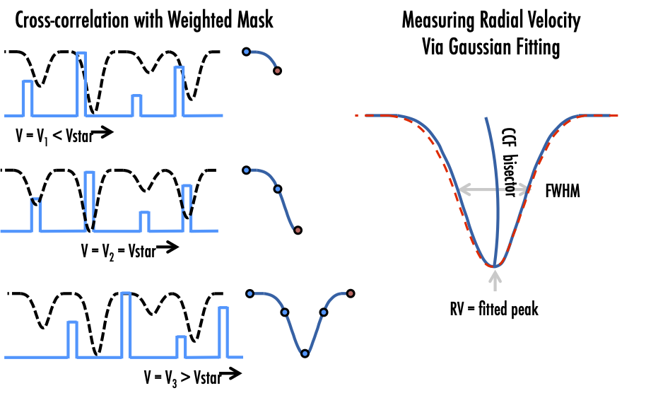
The extracted wavelength-calibrated spectra produced in level1 files are used to calculate the radial velocity (RV) of each observation. RVs are derived by cross correlating target spectra with a weighted numerical stellar mask based on spectral type (Baranne et al. 1996, Pepe et al. 2002). The NEID pipeline currently uses the public release of the ESPRESSO masks. While mask lines are historically selected empirically for RV stability, the mask width is set by the resolution of the instrument to cover approximately 1 pixel (in the case of NEID, this translates to 1km/s).
The cross correlation is performed in a corrected redshift space, which accounts for both the barycentric correction and the gamma velocity of the star. This centers the calculation around the peak of the cross-correlation function for each target, without requiring the exploration of a large span of redshift. Mask lines are also clipped at the edges to allow for the full barycentric throw of a star, to ensure that the same exact lines are always used for RV calculation of a target.
The module operates on each echelle order to produce individual cross-correlation functions (CCFs) that are stored in extension 12 of the level2 files. These are fit with Gaussians to produce order-by-order RV measurements that can be used to scrutinize chromatic behaviors. The order-by-order CCFs are then summed, and the sum is fit by a Gaussian to measure a single RV value for the observation. This aggregate value is stored in the level2 header, along with the corresponding measured uncertainty, and the BJD_TDB.
The order-by-order CCFs are then reweighted to their nominal observed spectral energy distribution expected in good conditions. These weights are derived by multiplying the measured system throughput by a black-body curve corresponding to the star’s temperature, and are reported in the CCFWTNNN keywords. The sum of these reweighted RVs, corresponding uncertainty, and BJD_TDB are stored in header keywords.
CCF Bisector Calculation
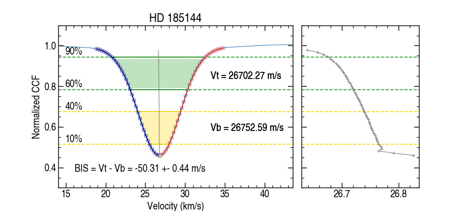
Bisector analysis is done on the combined CCFs in the velocity space to compute bisector inverse slope (BIS) value and its uncertainty (BISSUM, EBISSUM, BISMOD, and EBISMOD header keywords in extension 12 of Level2 files). BIS is difference between the velocity of the top (Vt) and bottom (Vb) sections of the line, with the top being the average mid-point of the flux levels located between 60 and 90% (green) and the bottom of those between 10 and 40% (yellow) of the line full depth. The BIS uncertainty is derived using the same method to obtain the CCF RV uncertainty, and is equal top and bottom velocity uncertainty added in quadrature.
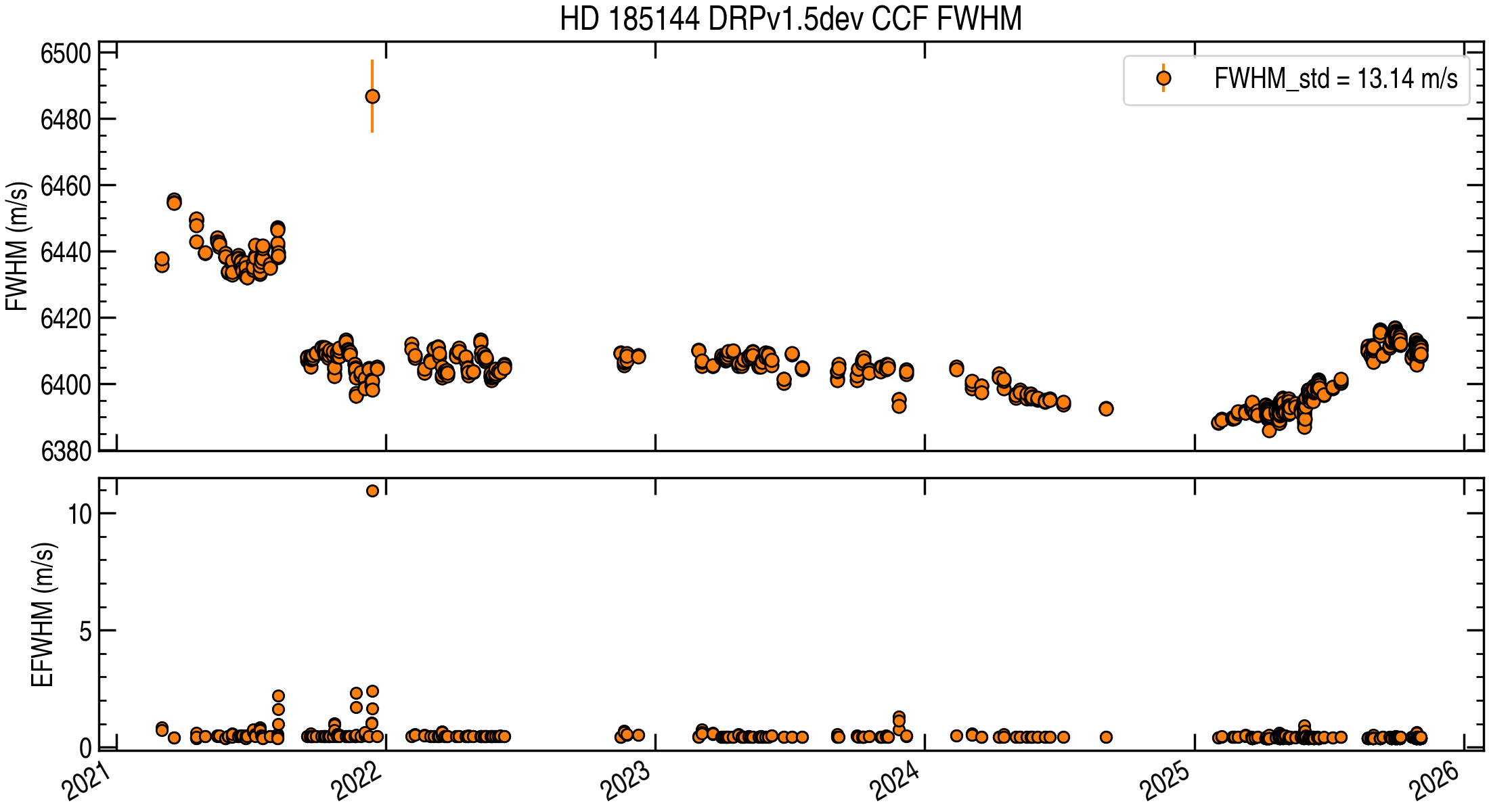
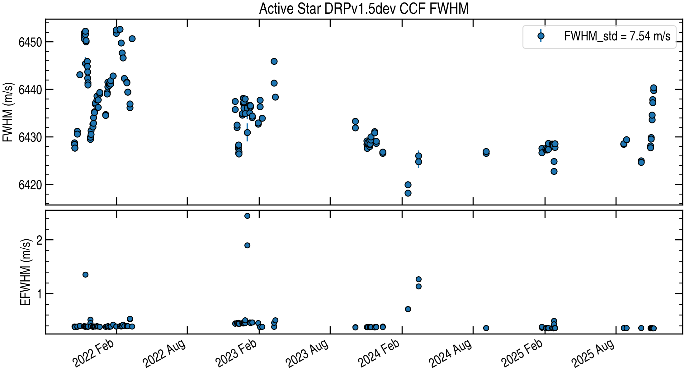
CCF FWHM and Uncertainty
The full width at half maximum (FWHM) for the cross-correlation function (CCF) is derived from the same Gaussian model fitted to the sampled CCF profile used for RVs. To estimate the uncertainty on the derived FWHM, the pipeline uses a Fisher-information (Cramer–Rao) approach based on the per-velocity-bin CCF uncertainties. This is the same information-content philosophy used to derive photon-noise-limited RV uncertainties (e.g., Bouchy et al. 2001).
Stitched 1D Spectra
Overview
NEID Level 2 files provide extracted echelle spectra as
multi-extension FITS data products. The primary science spectrum is
stored as 2D arrays with axes (order, pixel) for flux, variance,
and wavelength. Beginning in v1.5.0 the DRP also provides a 1D
stitched spectrum that combined all of the orders into a single
sequenced array. We believe the algorithms and derived products that
are described in this section are working well for normal NEID target
stars: main sequence FGKM stars with medium to high SNR. The DRP team
welcomes feedback from users on any issues they encounter with the
stitched spectra, particularly for targets falling outside of this
core parameter space.
Brifely, the stitching algorithm follows the following procedure:
constructing a normalized blaze correction (pixel-to-pixel blaze with an order-to-order lamp-envelope correction),
deblazing the science flux and propagating the variance,
resampling each order to a common wavelength grid with flux conservation and uncertainty propagation,
combining overlapping orders using inverse-variance weighting.
This product is intended for science use cases that benefit from a single 1D spectrum on a constant-velocity (log-wavelength) grid, while retaining a propagated uncertainty estimate.
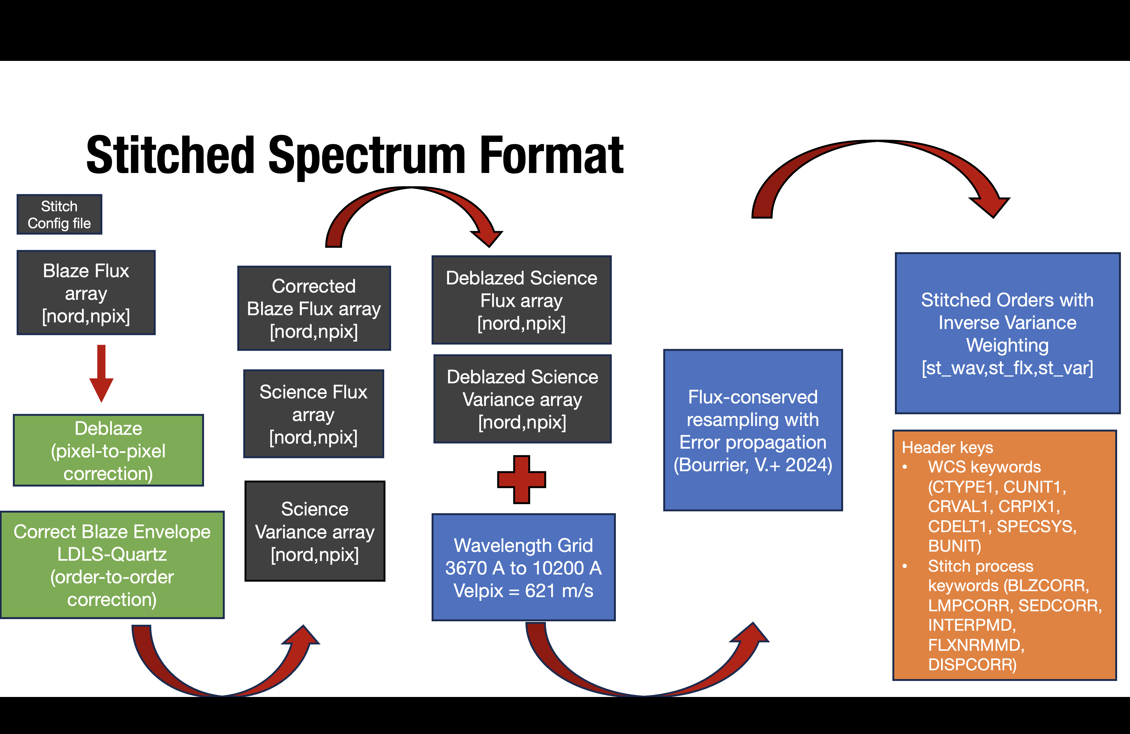
End-to-end workflow for stitched spectra generation.
Note
The stitched spectrum is derived from the Level 2 per-order extractions. It does not replace the native per-order arrays, and users should continue to rely on the original 2D products for applications that require strict order-by-order provenance or avoid resampling-induced correlations.
Inputs
Required Level 2 arrays (science fiber)
The stitcher uses the Level 2 extracted arrays (extension naming follows NEID conventions; exact extension names may vary with DRP versions and data level):
SCIFLUX: extracted science flux, shape(nord, npix), units of electrons.SCIVAR: extracted science variance, shape(nord, npix), units of electrons^2.SCIWAVE: wavelength solution, shape(nord, npix), vacuum wavelengths.SCIBLAZE: blaze / flat-relative response vector, shape(nord, npix).
Configuration file
A stitch configuration file defines:
global wavelength grid:
wavegrid_start,wavegrid_end(Angstrom), andvelpix(m/s)blue/red cotinuum sources order partition and smoothing ranges used for blaze-envelope estimation
echelle order index mapping of NEID extracted orders
Example plots of the relevant inputs (all orders):
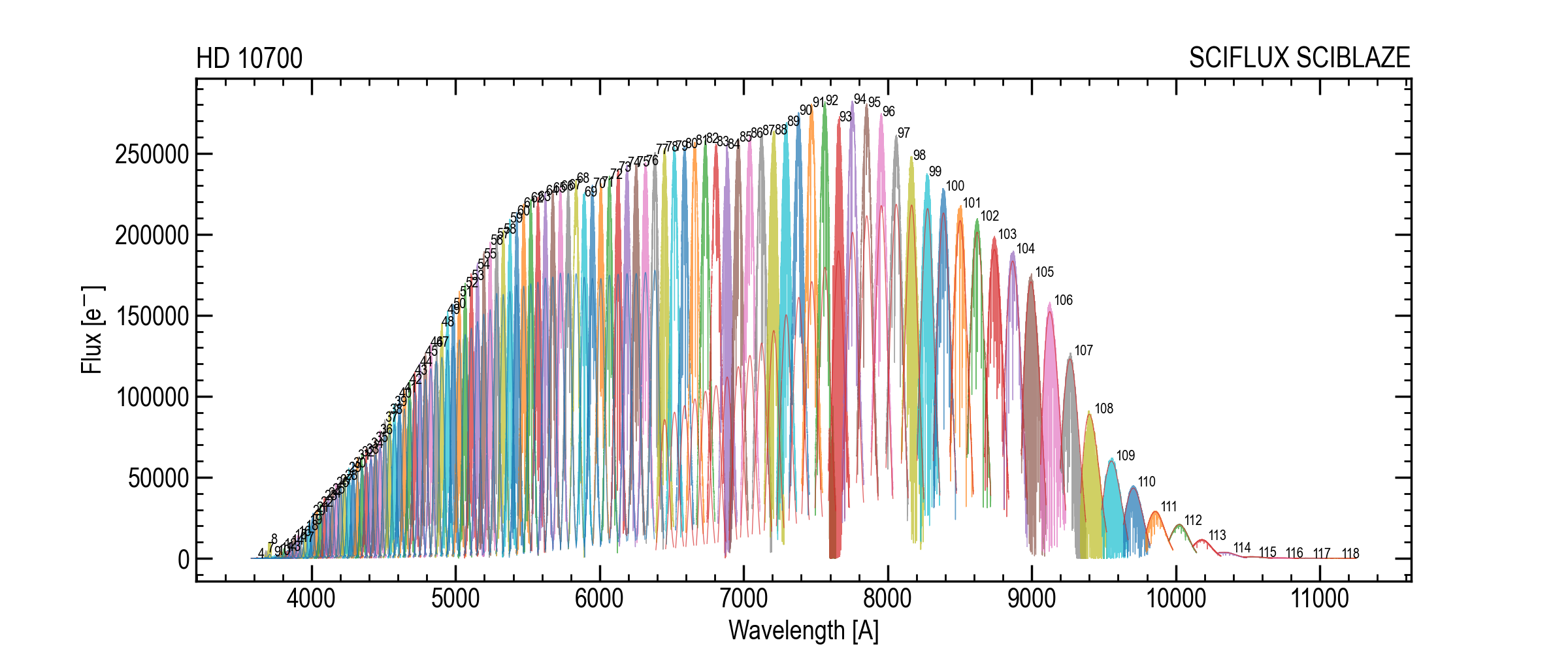
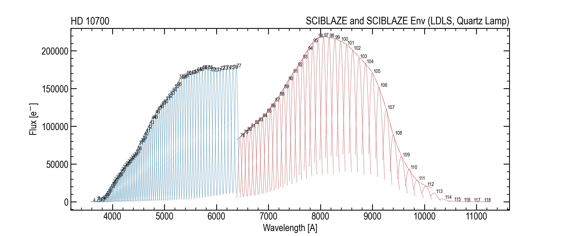
SCIFLUX and SCIBLAZE across all orders (example target).
Algorithm
1. Data quality masking
Pixels are masked prior to any modeling/resampling if they are non-finite, have non-positive variance, or fail additional user-defined quality criteria. Masking is carried through the resampling and stitching steps via order-by-order validity masks.
2. Blaze-envelope correction (order-to-order)
Continuum sources used in extraction are different blue and red orders (LDLS lamp for blue, quartz lamp for red). These lamps have different spectral energy distributions, and the extracted spectrum can retain low-frequency order-to-order structure associated with the illumination source and throughput trends. The stitcher estimates and removes a smooth order-to-order “blaze envelope” to isolate the pixel-scale blaze structure used for deblazing.
Method
For each order m:
define a robust order-level blaze statistic, a high percentile of
SCIBLAZEin the usable region,smooth the sequence of per-order values across order number using Savitzky–Golay filter,
interpolate the resulting envelope model back to pixel space to form
B_env[m, pix].
The envelope-corrected normalized blaze is:
Example envelope diagnostics:
Blaze envelope estimates for blue/red continuum sources (example).
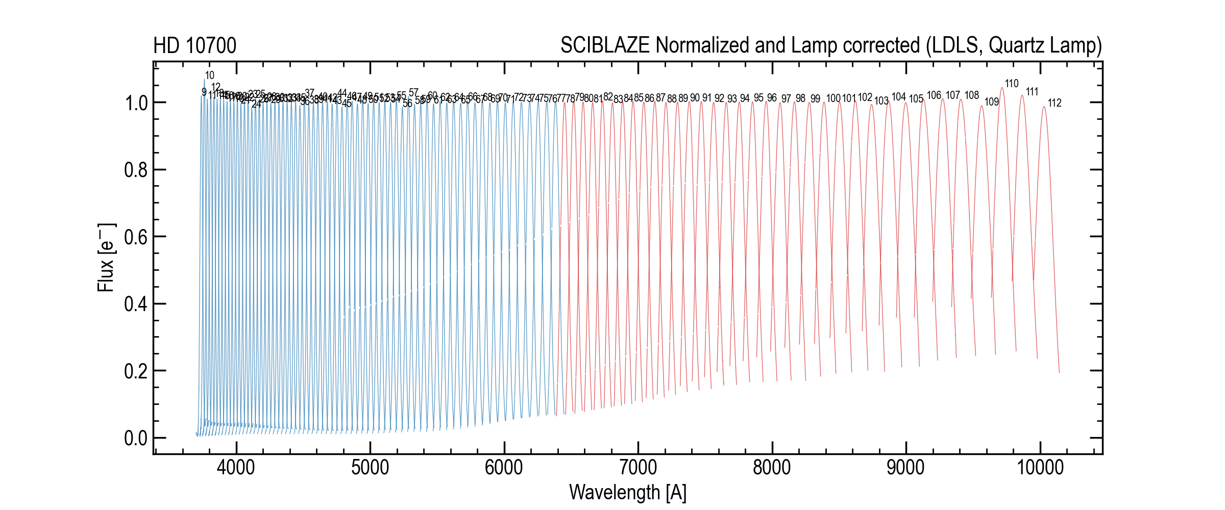
Envelope-corrected blaze model (example).
3. Deblazing and variance propagation
Science flux is deblazed with the normalized blaze, and the variance is propagated assuming the blaze model is noiseless relative to the science spectrum:
Example deblazed flux and variance (all orders):
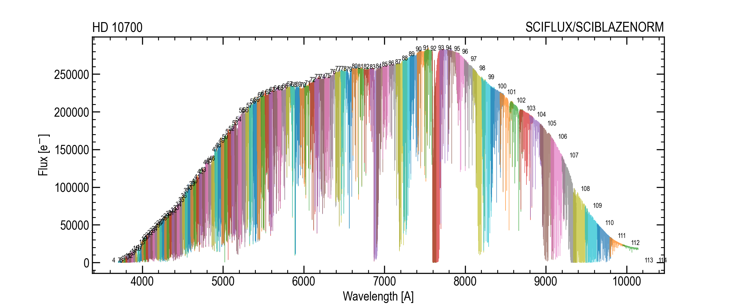
Deblazed SCIFLUX across all orders (example).
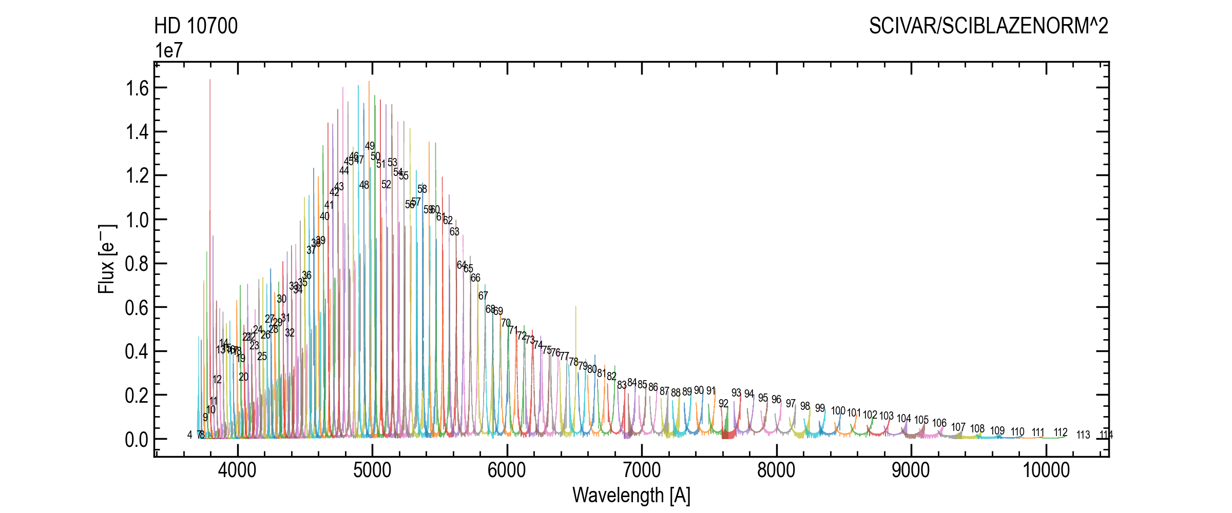
Deblazed SCIVAR across all orders (example).
4. Global stitched wavelength grid (constant velocity)
A single wavelength grid is constructed with constant spacing in \(\ln \lambda\),
corresponding to a constant velocity step velpix.
Let \(c\) be the speed of light and:
The grid spans [wavegrid_start, wavegrid_end] in vacuum Angstrom.
5. Flux-conserving resampling with uncertainty propagation (bindensity)
The stitcher resamples each order to the global grid using bindensity.resampling with
kind='cubic'. bindensity performs resampling by interpolating the cumulative in a way
that enforces conservation of the integral over each bin. The “cubic cumulative” mode is a
simplified cubic approach designed to reduce correlation in the resampled bins relative to
a full cubic spline (Bourrier, V. et al. 2024).
Key points
bindensityexpects bin edges for both the original and new grids.The input
yis a per-bin density, flux density per wavelength bin or flux density per pixel (current choice); the cumulative interpolation preserves integrated flux.If an input covariance is provided,
bindensityreturns the output covariance in the same lower-banded representation.
Variance-only input (diagonal covariance)
If only a variance array is available for the original bins, a diagonal covariance can be supplied
to bindensity in lower-banded form with bandwidth zero:
covhas shape(1, n)cov[0, i] = Var(y_i)
This avoids allocating or computing any dense (n, n) covariance matrix, while still enabling
bindensity to propagate uncertainties through the resampling step.
6. Stitching across orders (inverse-variance weighting)
After resampling, each wavelength bin may have contributions from multiple orders. The stitched flux is formed via inverse-variance weighting:
This naturally upweights the higher-S/N order in overlap regions (typically nearer the blaze peak) and downweights noisier order edges.
Overlap diagnostics
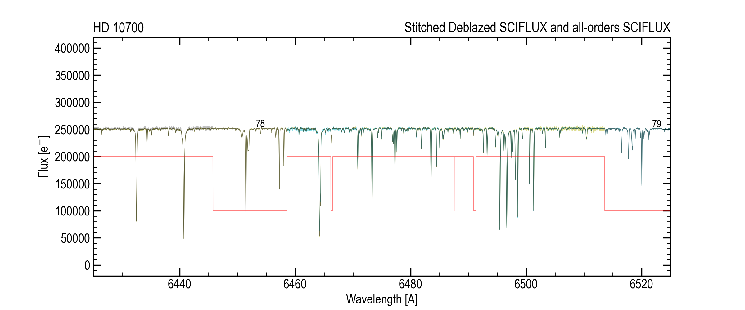
Stitched deblazed spectrum with order contributions (example zoom).
Variance-weighted vs. unweighted comparison
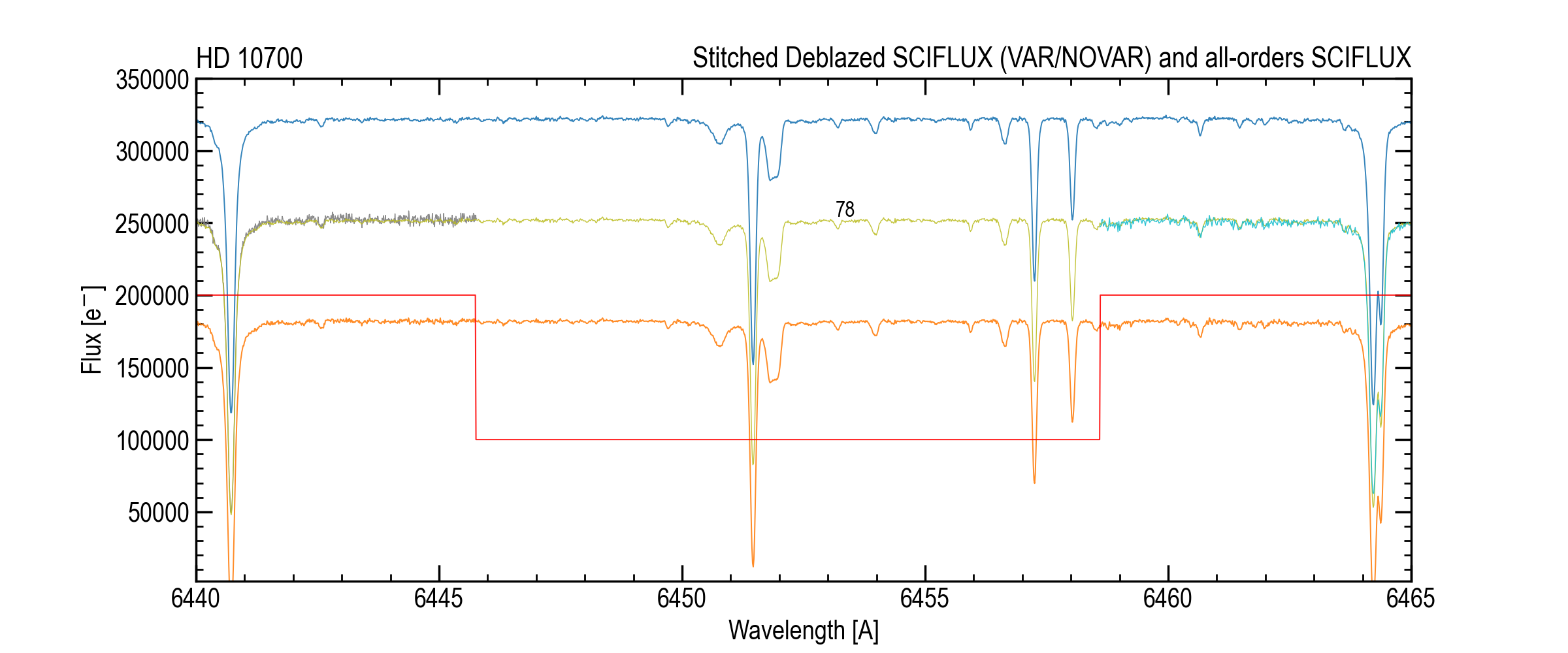
Comparison of stitched results with/without variance weighting.
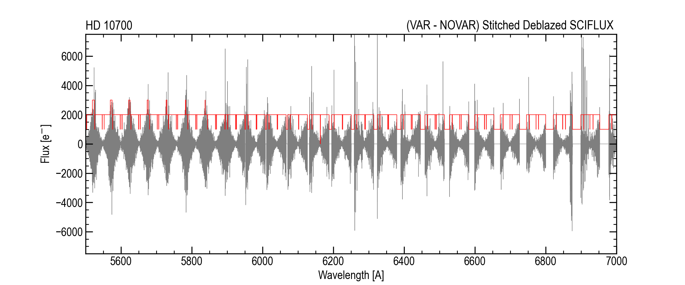
Difference (VAR - NOVAR) to highlight overlap behavior.
Output: New HDUs in the Stitched Level 2 File
The stitcher writes the original Level 2 HDUs unchanged and appends new extensions for the stitched product.
Stitched arrays
The stitched spectrum is stored as three 1D arrays of length nwave:
SCIWAVESTITCH(float64): stitched wavelength grid, vacuum AngstromSCIFLUXSTITCH(float64): stitched deblazed flux on the stitched grid (electrons)SCIVARSTITCH(float64): stitched propagated variance (electrons^2)
Note
The stitched spectrum is provided in vacuum wavelengths, consistent with NEID Level 1/2 wavelength conventions. The variance is a diagonal uncertainty estimate for the stitched spectrum; resampling can introduce inter-pixel covariance that is not currently saved.
Header keywords for the stitched WCS
The stitched wavelength grid is described with a 1D spectral WCS. The header set includes:
CTYPE1:'WAVE-LOG'(log-lambda sampling)CUNIT1:'Angstrom'CRVAL1: starting wavelengthCRPIX1: reference pixel (1-indexed)CDELT1: step in log-lambdaSPECSYS:'BARYCENT'BUNIT: units of the stitched flux array
Processing provenance keywords
The stitcher writes boolean/string keywords documenting the processing chain:
BLZCORR: blaze correction applied?LMPCORR: lamp-SED-envelope correction applied?SEDCORR: order-to-order Stellar SED correction applied?INTERPMD: resampling/interpolation method of input spectrum (e.g.'BINDENSITY')FLXNRMMD: flux normalization methodDISPCORR: has wavelength dispersion been corrected?
How to use the new HDUs
List extensions and inspect the stitched spectrum
from astropy.io import fits

fn = "neidL2_YYYYMMDDThhmmss_stitched.fits"

with fits.open(fn) as hdul:
    hdul.info()

    wave = hdul["SCIWAVESTITCH"].data
    flux = hdul["SCIFLUXSTITCH"].data
    var  = hdul["SCIVARSTITCH"].data

# Basic sanity checks
assert wave.ndim == 1
assert flux.shape == wave.shape
assert var.shape  == wave.shape

snr = flux / var**0.5
Plot a region of the stitched spectrum
import numpy as np
import matplotlib.pyplot as plt

w1, w2 = 6440.0, 6465.0
m = (wave >= w1) & (wave <= w2)

plt.figure()
plt.plot(wave[m], flux[m], lw=1)
plt.xlabel("Wavelength [Angstrom]")
plt.ylabel("Flux [e-]")
plt.title("Stitched spectrum (zoom)")
plt.show()
Compare stitched 1D to native order data
from astropy.io import fits
import numpy as np

fn = "neidL2_YYYYMMDDThhmmss_stitched.fits"

with fits.open(fn) as hdul:
    wav2d  = hdul["SCIWAVE"].data      # (nord, npix)
    flx2d  = hdul["SCIFLUX"].data
    var2d  = hdul["SCIVAR"].data

    wave1d = hdul["SCIWAVESTITCH"].data
    flux1d = hdul["SCIFLUXSTITCH"].data
    var1d  = hdul["SCIVARSTITCH"].data

# Example: locate where a given order overlaps a stitched region
ord_idx = 78
wmin, wmax = np.nanmin(wav2d[ord_idx]), np.nanmax(wav2d[ord_idx])
m = (wave1d >= wmin) & (wave1d <= wmax)

# 'm' marks stitched pixels covered by this order's wavelength span (coarse QA).
# For detailed QA, use the per-order resampled maps if provided (RESAMPFLUX/RESAMPMASK).
RV Header information
The RVs are stored in header keywords in Level 2 extension 12:
CCFJDSUM BJD_TDB for the summed RV
CCFRVSUM Barycentric corrected RV for summed orders
DVRMS Calculated uncertainty on CCFRVSUM
FWHMSUM FWHM derived from the summed CCF fit (New in DRPv1.4.0)
EFWHMSUM FWHM uncertainty from the summed CCF fit (New in DRPv1.5.0)
BISSUM BIS value calculated from the summed CCF Bisector (New in DRPv1.4.0)
EBISSUM BIS uncertainty calculated from the summed CCF Bisector (New in DRPv1.4.0)
FITSUMFN Function fit to CCFSUM. Default is Gaussian-with-offset (New in DRPv1.4.0)
FITSUMV0 Offset parameter (ct) of CCFSUM Gaussian-with-offset fit (New in DRPv1.4.0)
FITSUMV1 Mean (CCFRVSUM) parameter (km/s) of CCFSUM Gaussian-with-offset fit (New in DRPv1.4.0)
FITSUMV2 Standard dev. parameter (km/s) of CCFSUM Gaussian-with-offset fit (New in DRPv1.4.0)
FITSUMV3 Amplitude parameter (ct) of CCFSUM Gaussian-with-offset fit (New in DRPv1.4.0)
CCFJDMOD BJD_TDB for the reweighted RV
CCFRVMOD Barycentric corrected, reweighted, summed RV
DVRMSMOD Calculated uncertainty on CCFRVMOD
FWHMMOD FWHM derived from the weighted CCF fit (New in DRPv1.4.0)
EFWHMMOD FWHM uncertainty from the weighted CCF fit (New in DRPv1.5.0)
BISMOD BIS value calculated from the weighted CCF Bisector (New in DRPv1.4.0)
EBISMOD BIS uncertainty calculated from the weighted CCF Bisector (New in DRPv1.4.0)
FITMODFN Function fit to CCFMOD. Default is Gaussian-with-offset (New in DRPv1.4.0)
FITMODV0 Offset parameter (ct) of CCFMOD Gaussian-with-offset fit (New in DRPv1.4.0)
FITMODV1 Mean (CCFRVMOD) parameter (km/s) of CCFMOD Gaussian-with-offset fit (New in DRPv1.4.0)
FITMODV2 Standard dev. parameter (km/s) of CCFMOD Gaussian-with-offset fit (New in DRPv1.4.0)
FITMODV3 Amplitude parameter (ct) of CCFMOD Gaussian-with-offset fit (New in DRPv1.4.0)
CCFWTNNN Reweight factor for order NNN used in deriving the MOD values
CCFRVNNN Barycentric corrected RV for order NNN
CCFZNNN Barycentric corrected redshift for order NNN
The NEID team recommends that users of v1.1.0 data use CCFRVMOD velocities
Stellar Activity Info
Calculation of the activity index
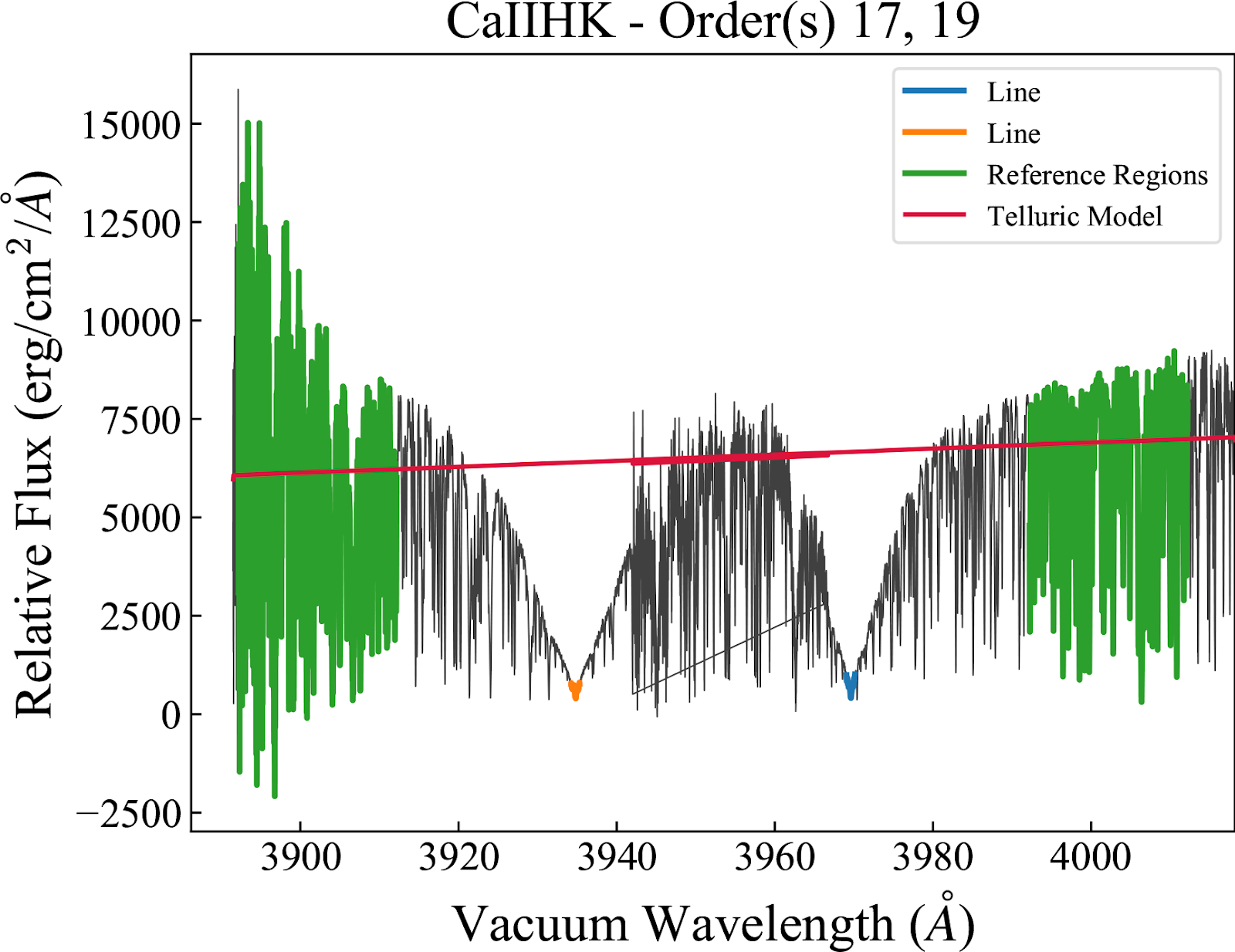
The activity module is run on the Level 2 files. We use each observed spectrum’s blaze function (output by the flat relative optimal extraction) to convert the raw flux to relative specific flux. We also use the telluric model described above to remove telluric absorption from the observed spectrum.
An activity index is a ratio of the average flux in a line or set of lines to the average flux in a pair of reference regions (bluer and redder than the lines used). We use a combination of the algorithms described in Zechmeister et al. 2018 (2018A&A…609A..12Z) and Appendix A of Gomes da Silva et al. 2021 (2021A&A…646A..77G) to calculate:
the total integrated flux inside a given bandpass (GdS Equation A.2)
errors on the flux using the measured variance (GdS Equation A.3)
indices given a set of sensitivty lines and reference regions (Z Equation 27). Note that for features with more than one sensitive lines (such as Ca II H&K), the numerator is the average flux across both line cores. The denominator is the average of the two reference region fluxes.
error of the index assuming error propagation and ignoring covariances (Z Equation 29 and GdS Equation A.5).
We interpolate the flux, wavelength, and variance arrays prior to the calculation to account for any pixel shifts in the wavelength.
(i) and (ii) above are calculated for all overlapping orders where the given bandpass is available, which are then averaged via a weighted mean for each line and reference region. To maintain flux agreement between overlapping orders, the flux in each order is scaled by the original mean step size for that order, which is performed at the interpolation step. Likewise, the variance is scaled by the original mean step size squared.
Indices are calculated for spectra both with and without the telluric correction applied. Both values are provided in the activity extension table described below.
Note 1: Three major changes to the calculation described above were added in DRP v1.4.0:
raw flux is converted to relative specific flux using the per-frame blaze function rather than the instrumental throughput model.
the telluric model is used for removing telluric absorption.
step (iii) above now averages together the line core and reference region fluxes rather than summing.
The use of the per-frame blaze removes significant offsets in activity index values reduced with DRP v1.2 and v1.3 introduced by time-varying instrumental throughput models. While data in different RV eras should still be treated as separate data sets, this change has standardized activity indices across the NEID lifetime.
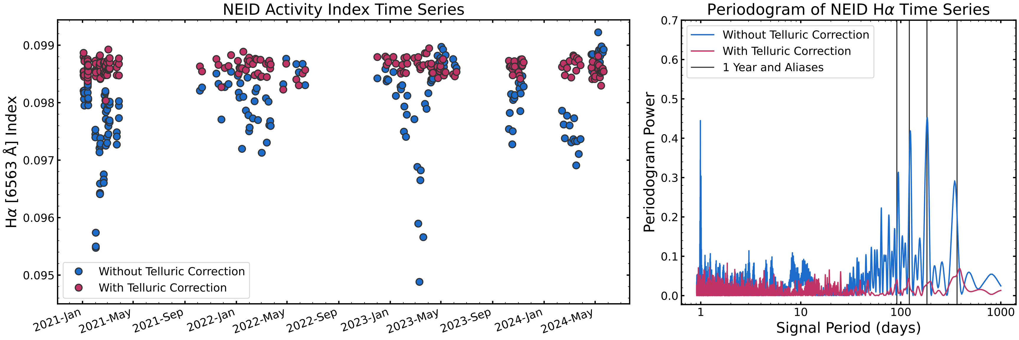
The telluric correction reduces scatter in activity index time series introduced when telluric absorption lines are present in the spectral regions used to calculate indices. The plot below shows the H-alpha time series for NEID observations of a star with and without telluric correction applied. The telluric corrected values are much more stable, and a strong, spurious yearly signal in the non-telluric corrected values (seen in the periodogram to the right) is reduced when the telluric absorption is removed. That yearly signal is caused by telluric-introduced noise from barycentric motions throughout the year.
The change from summing to averaging in step (iii) has removed a factor of 2 difference seen between activity index values calculated with the NEID DRP and SERVAL.
Activity Index Definition
We calculate the following activity indices:
Ca II H&K (S-index) We follow the definition from Duncan et al. 1991 (1991ApJS…76..383D). This S-index is not calibrated to match the observations from HKP-1 (Wilson 1978; 1978ApJ…226..379W) such that in Equation 1 of Duncan et al. 1991, the constant of proportionality is unity (alpha==1). When calculating the average integrated flux in the lines, we adopt a triangular weighting function to the lines with a FWHM of 1.09 Angstroms to mimic the measured instrumental response profiles of the H and K channels from Duncan et al. 1991. The average integrated flux in the reference regions is calculated adopting a simple box weighting function. “CaIIHK” in the activity table.
He I D3 line We follow the definition from Gomes da Silva et al. 2011 (2011A&A…534A..30G). “HeI_1”/”HeI_2” in the activity table.
Na I D1/D2 lines We follow the definition from Gomes da Silva et al. 2011. “NaI” in the activity table.
H-alpha We follow the definition from Gomes da Silva et al. 2011 and calculate the index with both a 0.6 Angstrom or 1.6 Angstrom window centered on the line. “Ha06_1”/”Ha06_2”/”Ha16_1”/”Ha16_2” in the activity table.
Ca I We follow the definition from the ACTIN code (Gomes da Silva et al. 2018; 2018JOSS….3..667G) and include this line as an activity insensitive line. “CaI_1”/”CaI_2” in the activity table.
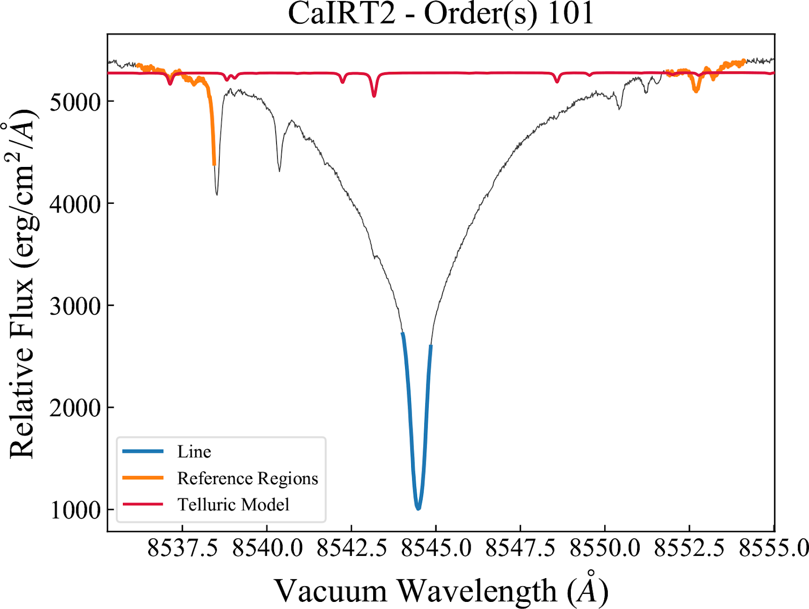
Ca II Infra-red Triplet We follow the definition used in the SERVAL pipeline (Zechmeister et al. 2018; 2018A&A…609A..12Z). There are three separate indices centered on the Ca II lines at 8498.018, 8542.089, and 8662.14 Angstroms. “CaIRT1”/”CaIRT2”/”CaIRT3” in the activity table.
Na I NIR Doublet We follow the definition from Table 1 of Robertson et al. 2016 (2016ApJ…832..112R). “NaINIR” in the activity table.
Paschen Delta We follow the definition from Table 1 of Robertson et al. 2016. “PaDelta” in the activity table.
Mn I (539.4 nm) There is no standard defining this line. We extrapolate from Danilovic, et al. 2016, using the reference window of 539.491 nm defined there. The second reference region is the mirror of that wavelength on the other side of the line. “Mn539” in the activity table
CCF Bisector Inverse Slope Bisector inverse slope value (BIS) [km/s] measures the slope between the derived midpoint of the top 30%-tile of the CCF relative to the bottom 30%-tile (Queloz et al. 2001; 2001A&A…379..279Q). The weighted CCF (CCFMOD) is used for this index.
CCF FWHM The full width at half maximum (FWHM) of the CCF, derived the Gaussian model fitted to the sampled CCF profile. The weighted CCF (CCFMOD) is used for this index.
Activity Table Description
A table of index values and additional information can be accessed by reading the Level 2 extension called “ACTIVITY”. All reference wavelengths are listed in air wavelengths. The table contains the following columns:
INDEX, the name of the index calculated.
A subscript of “_tellcorr” appended to the end of the index name means that the value in that row was calculated after the telluric correction was applied to the observed spectrum.
A subscript of “_1” or “_2” is a deprecated feature; both values are calculated in an identical manner and the values are duplicates of each other.
VALUE, the value of the activity index using the algorithms described above
UNCERTAINTY, the uncertainty of the activity index using the algorithms described above
LINE_CENTER, the line center(s) used to calculate the flux in the sensitivity lines
LINE_WIDTH, the width of the window used to calculate the flux in the sensitivity lines. If multiple lines are used in the calculation, this represents the window used around each line.
REF_CENTER1, the center of the blue reference region
REF_CENTER2, the center of the red reference region
REF_WIDTH1, the width of the window used to calculate the flux in the blue reference region
REF_WIDTH2, the width of the window used to calculate the flux in the red reference region
STATUS, a string for containing comments regarding the reduction, in v1.1.0 this is always empty
Note 1: Starting with DRPv1.4.0, each line index has two rows in the
table for two different calculations: with and without the telluric
correction. The difference is noted in the INDEX column value: the
calculation with the correction has “_tellcorr” added to the index name
while the calculation without does not.
The telluric corrected and non-telluric corrected values for the Ca II H&K and Paschen Delta indices in DRPv1.4 are the same. This is because no telluric model is defined outside of zero-indexed spectral orders 55-110, and these spectral features fall outside that range.
Note 2: Starting with DRPv1.5.0, the CCF BIS and FWHM indices have been
added to the activity table. These indices are derived from the weighted CCF
(CCFMOD) and not from spectral line fluxes, only INDEX, VALUE, and
UNCERTAINTY columns are populated for these rows.
Caveats
Some index values and the uncertainties may be negative because some extracted 1D spectra have negative values (see extraction section). We do not mask out negative values while calculating the integrated flux to limit any bias in the activity index. Negative values are typically seen when calculating the index of a low S/N spectrum. We also perform no correction for seeing effects when calculating the activity indices.
DRP v1.4.0 now corrects telluric absorption of the observed spectrum prior to calculating indices. While we recommend use of the telluric corrected index values, we note that the telluric correction is not perfect. There may be remaining telluric-caused signals in activity index time series.
Major Algorithm Update History
DRPv1.3.0 Update:
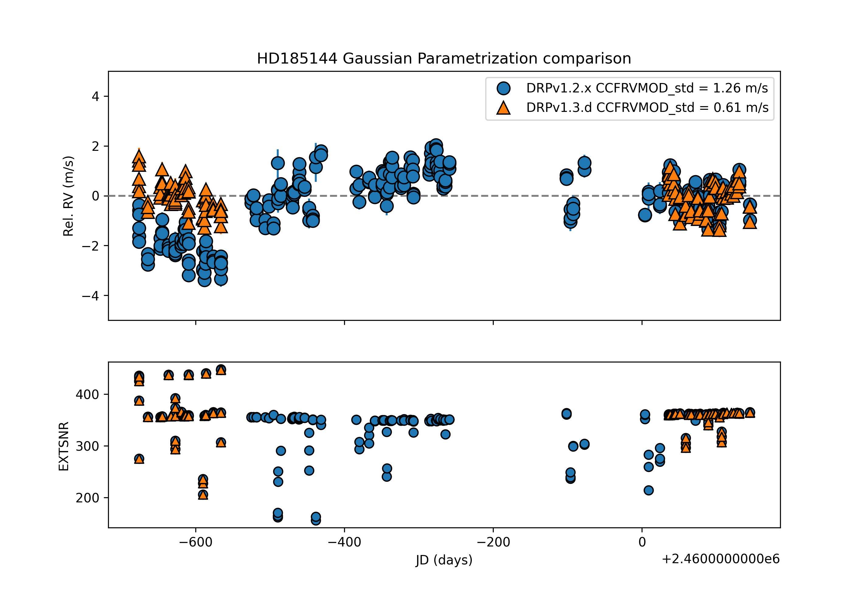
1) Change of the CCF Gaussian fit function parametrization. The Gaussian function has been re-parametrized to include an offset term. The offset initial guess has been set to be the median of the CCF. In versions < DRPv1.3.0 the median of the CCF was subtracted from the input CCF to allow the fitter work. This re-parametrization allows the fit and output to maintain the input CCF flux scale, which is useful for future analysis of the CCF fit parameters. The Gaussian re-parametrization update provides similar or lower scatter in the RVs, as shown below in Sigma Dra (note that an offset has been removed in this plot to account for the Contreras fire instrument reset).
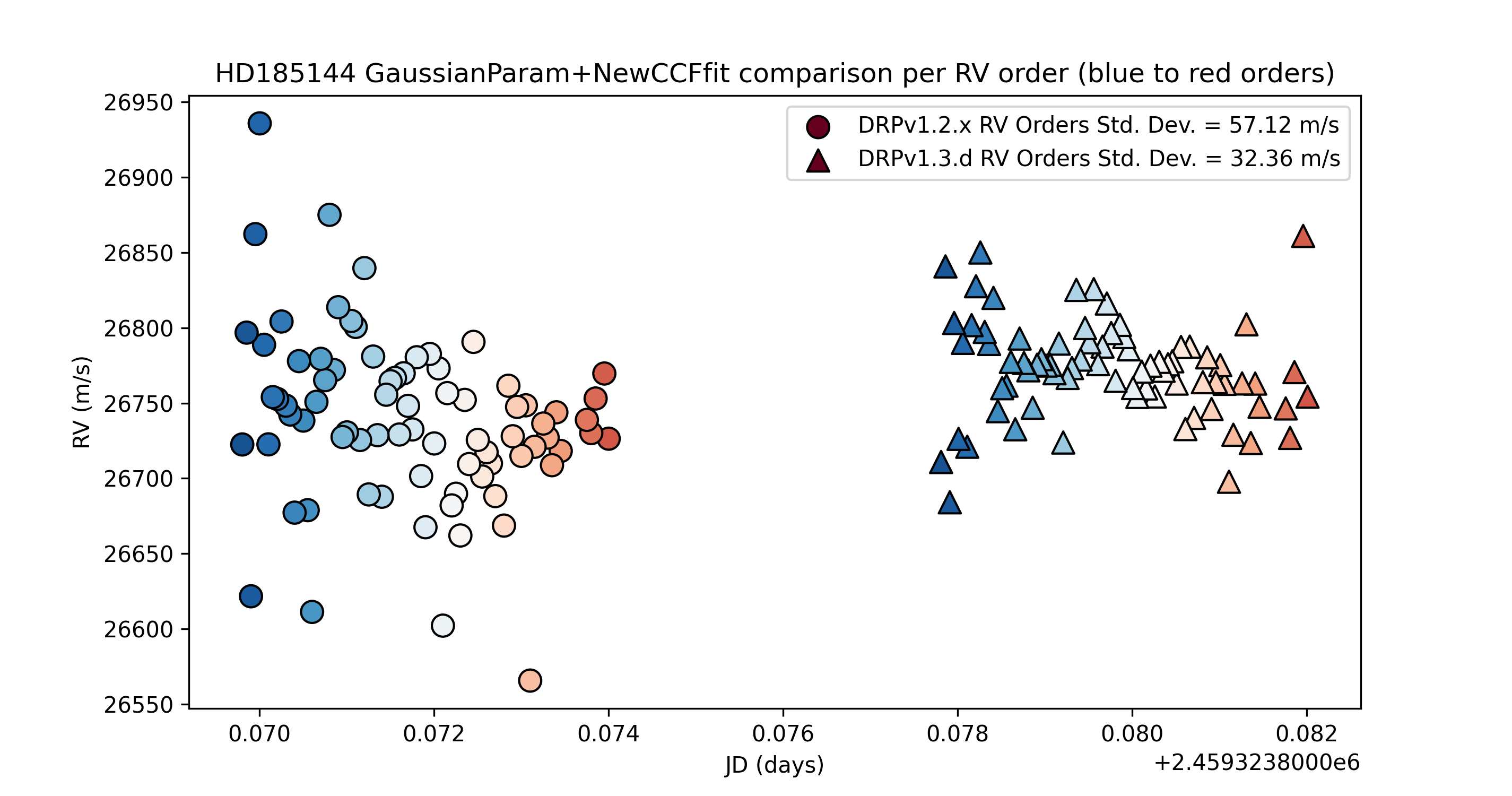
2) Added weights to the CCF Gaussian fitter to make the fit more accurate in the core compared to the wings. An CCF error array is created from the input CCF to force the CCF fitter to priorize fit accuracy in the core of the CCF, where the RV is derived, rather than the wings of the CCF. The update is currently only applied to fits to the individual order CCFs; the sum and sum-weighted CCF arrays are unchanged. The update to the Gaussian fitter decrease about 2 times the scatter of the order-by-order RVs by removing systematic offsets that affected previous individual order fits, as shown below for Sigma Dra.
DRPv1.4.0 Update:
Added Bisector Inverse Slope (BIS) calculation and its uncertainty from CCF.
Added fitting parameters derived from the function fit for the summed and weighted CCFs.
Added FWHM derived from fitting parameters of the summed and weighted CCFs.
DRPv1.5.0 Update:
Added stitched 1D spectrum product to Level 2 files.
Added FWHM uncertainty derived from fitting parameters of the summed and weighted CCFs.
Last Updated: 2026-01-26, JKL, DMK, CFB, LAP